Preface
Recently, I have been working on a small driver for ambient lighting using 12V LED strips like you can get
inexpensively from China. I wanted to be able to just throw one of these somewhere, stick down some LED tape, hook it up
to a small transformer and be able to control it through Wifi. When I was writing the firmware, I noticed that when
fading between different colors, the colors look all wrong! This observation led me down a rabbit hole of color
perception and LED peculiarities.
The idea of the LED driver was that it can be used either with up to eight single-color LED tapes or, much more
interesting, with up to two RGB or RGBW (red-green-blue-white) LED tapes. For ambient lighting high color resolution was
really important so you could dim it down a lot without flickering. I ended up using the same driver stage I used in the
multichannel LED driver project for its great color resolution and low hardware requirements.
 An illustration of the RGB color cube.
Picture by
Maklaan from Wikimedia Commons,
CC-BY-SA 3.0
An illustration of the RGB color cube.
Picture by
Maklaan from Wikimedia Commons,
CC-BY-SA 3.0
To make setting colors over Wifi more intuitive I implemented support for HSV colors. RGB is fine for communication
between computers, but I think HSV is easier to work with when manually inputting colors from the command line. RGB is
close to how most monitors, cameras and the human visual apparatus work on a very low level but doesn't match
higher-level human color perception very well. When we describe a color we tend to think in terms of "hue" or
"brightness", and computing a measure of those from RGB values is not easy.
Colors and Color Spaces
Color spaces are a mathematical abstraction of the concept of color. When we say "RGB", most of the time we actually
mean sRGB, a standardized notion of how to map three numbers labelled "red", "green" and "blue" onto a perceived
color. HSV is an early attempt to more closely align these numbers with our perception. After HSV, a number of other
perceptual color spaces such as XYZ (CIE 1931) and CIE Lab/LCh were born, further improving this alignment. In
this mathematical model, mapping a color from one color space into another color space is just a coordinate
transformation.
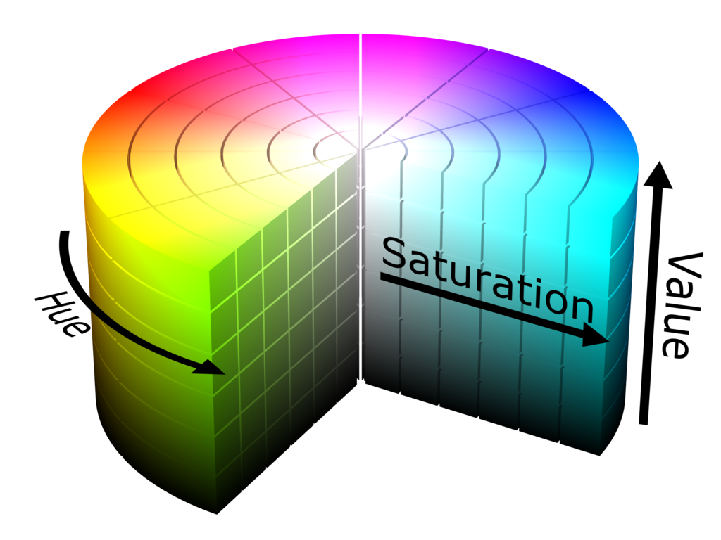 An illustration of the HSV color space as a cylinder.
Picture by
SharkD from Wikimedia Commons,
CC-BY-SA 3.0
An illustration of the HSV color space as a cylinder.
Picture by
SharkD from Wikimedia Commons,
CC-BY-SA 3.0
CIE 1931 XYZ is much larger than any other color space, which is why it is a good basis to express other color spaces
in. In XYZ there are many coordinates that are outside of what the human eye can perceive. Below is an illustration of
the sRGB space within XYZ. The wireframe cube is (0,0,0) to (1,1,1) in XYZ. The colorful object in the middle is what
of sRGB fits inside XYZ, and the lines extending out from it indicate the space that can be expressed in sRGB but not in
XYZ. The fat white curve is a projection of the monochromatic spectral locus, that is the curve of points you get in
XYZ for pure visible wavelengths.
As you can see, sRGB is much smaller than XYZ or even the part within the monochromatic locus that we can perceive. In
particular in the blues and greens we loose a lot of colors to sRGB.
Illustration of the measured sRGB color space within XYZ. The thick, white line is the spectral
locus.
mkv/h264 download /
webm download
The wrong colors I got when fading between colors were caused by this coordinate transformation being askew. Thinking
over the problem, there are several sources for imperfections:
- The LED driver may not be entirely linear. For most modulations such as PWM the brightness will be linear starting
from a certain value, but there is probably an offset caused by imperfect edges of the LED current. This offset can be
compensated with software calibration. I built a calibration setup for driver linearity in the multichannel LED
driver project. Below are pictures of ringing on the edges of an LED driver's waveform.
- The red, green and blue channels of the LEDs used on the LED tape are not matched. This skews the RGB color space.
In practice, the blue channel of my RGB tape to me looks much brighter than the red channel.
- The precise colors of the red, green and blue channels of the LEDs are unknown. Though the red channel looks red, it
may be of a slightly different hue compared to the reference red used in sRGB which would also skew the RGB color
space.
These last two errors are tricky to compensate. What I needed for that was basically a model of the perceived colors
of the LED tape's color channels. A way of doing his is to record the spectra of all color channels and then evaluate
their respective XYZ coordinates. If all three channels are measured in one go with the same setup the relative
magnitudes of the channels in XYZ will be accurate.
To map any color to the LEDs, the color's XYZ coordinates simply have to be mapped onto the linear coordinate system
produced by these three points within XYZ. LEDs are mostly linear in their luminous flux vs. current characteristic so
this model will be adequate. The spectral integrals mapping the channels' measured responses to XYZ need only be
calculated once and their results can be used as scaling factors thereafter.
Measuring the spectrum
In order to compensate for the cheap LED tape's non-ideal performance I had to measure the LED's red, green and blue
channels' spectra. The obvious thing would be to go out and buy a spectrograph, or ask someone to borrow theirs. The
former is kind of expensive, and I did not want to wait two weeks for the thing to arrive. The latter I could probably
not do every time I got new LED tape. Thus the only choice was to build my own.
Luckily, building your own spectrometer is really easy. The first thing you need is something that splits incident light
into its constituent wavelengths. In professional devices this is called the `monochromator`_, since it allows extraction
of small color bands from the spectrum. The second thing is some sort of optics that project the incident light onto a
screen behind the monochromator. In professional devices lenses or curved mirrors are used. In a simple homebrew job a
pinhole as you would use in a camera obscura does a remarkably nice job.
For the monochromator component several things could be used. A prism would work, but I did not have any. The
alternative is a diffraction grating. Professional gratings are quite specialized pieces of equipment and thus
rather expensive. Luckily, there is a common household item that works almost as well: A regular CD or DVD. The
microscopic grooves that are used to record data in a CD or DVD work the same as the grooves in a professional
diffraction grating.
Household spectra
From this starting point, a few seconds on my favorite search engine yielded an article by two researchers from the
National Science Museum in Tokyo providing a nice blueprint for a simple cardboard-and-DVD construction for use in
classrooms. I replicated their device using a DVD and it worked beautifully. Daylight and several types of small LEDs I
had around did show the expected spectra. Small red, yellow, green, and blue LEDs showed narrow spectra, daylight one
continuous broad one, and white LEDs a continuous broad one with a distinct bright spot in the blue part. The
single-color LED spectra are quite narrow since they are determined by the LED's semiconductor's band gap, which is
specific to the semiconductor used and is quite precise. White LEDs are in fact a blue LED chip covered with a so-called
phosphor. This phosphor is not elementary phosphorus but an anorganic compound that absorbs the LED chip's blue light
and re-emits a broader spectrum of more yellow-ish wavelengths instead. The final LED spectrum is a superposition of
both spectra, with some of the original blue light leaking through the phosphor mixing with the broadband yellow
spectrum of the phosphor.
Now that I had a spectrograph, I needed a somewhat predictable way of measuring the spectrum it gave me.
Measuring a spectrum
Pointing a camera at the spectrograph would be the obvious thing to do. This produces pretty images but has one critical
flaw: I wanted to acquire quantitative measurements of brightness across the spectrum. Since I don't have a precise
technical datasheet specifying the spectral response of any of my cameras I can't compare the absolute brightness of
different colors on their pictures. Some other sensor was needed.
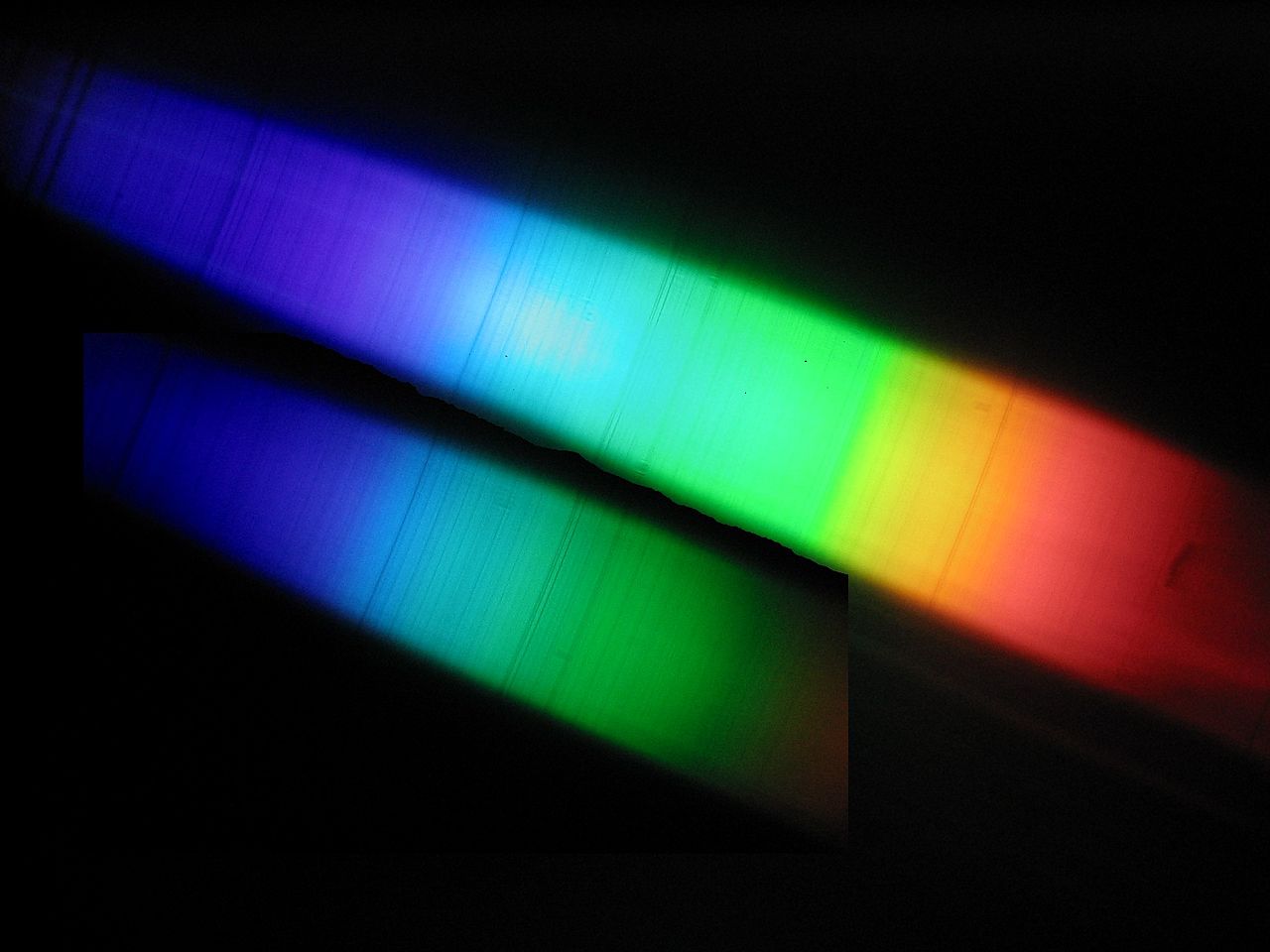 The daylight spectrum as seen using a DVD as a grating.
Picture by
Xofc from Wikimedia Commons,
CC-BY-SA 4.0
The daylight spectrum as seen using a DVD as a grating.
Picture by
Xofc from Wikimedia Commons,
CC-BY-SA 4.0
Measuring light intensity
Looking around my lab, I found a bag of SFH2701 visible-light photodiodes. Their
datasheet includes their spectral response so I can compensate for that, allowing precise-ish absolute intensity
measurements. Just like LEDs, photodiodes are extremely linear across several orders of magnitude. The datasheet of the
classic BPW34 photodiode shows that this photodiode's light current is exactly proportional to illuminance over at
least three orders of magnitude. The SFH2701 datasheet does not include a similar graph but its performance will be
similar. The SFH2701 photodiodes I had at hand were perfect for the job compared to the vintage BPW34 since their
active sensing area is really small (0.6mm by 0.6mm) compared to the BPW34 (a whopping 3mm by 3mm). If I were to use a
BPW34 I would have to insert some small apterture in front of it so it does not catch too broad a part of the
spectrum at once. The SFH2701 is small enough that if I just point it at the projected spectrum directly I will
already get only a small part of the spectrum inside its 0.6mm active area.
To convert the photodiode's tiny photocurrent into a measurable voltage I built another copy of the transimpedance
amplifier circuit I already used in the multichannel LED driver. A transimpedance amplifier is an
amplifiert that produces a large voltage from a small current. The weird name comes from the fact that it works kind of
like an amplified resistor (which can be generalized as an impedance electrically). Apply a current to a resistor and
you get a voltage. A transimpedance amplifiert does the same with the difference that its input always stays at 0V,
making it look like an ideal current sink to the connected current source.
Transimpedance amplifiers are common in optoelectronics to convert small photocurrents to voltages. In this instance I
built a very simple circuit with a dampened transimpedance amplifier stage followed by a simple RC filter for noise
rejection and a regular non-inverting amplifier using another op-amp from the same chip to further boost the filtered
transimpedance amplifier output. I put all the passives setting amplifier response (the gain-setting resistors and the
filter resistor and capacitors) on a small removable adapter so I could easily change them if necessary. I put a small
trimpot on the virtual ground both amplifers use as a reference so I could trim that if necessary.
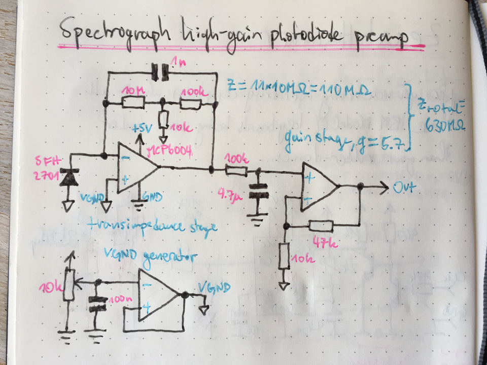 The photodiode preamplifier schematic. Schematic drawn with an unlicensed copy of
DaveCAD.
The photodiode preamplifier schematic. Schematic drawn with an unlicensed copy of
DaveCAD.
Following are pictures of the preamplifier board. The connectors on the top-left side are two copies of the analog
signal for the ADC and a small panel meter. The SMA connector is used as the photodiode input since coax cables are
generally low-leakage and have built-in shielding. The circuit is powered via the micro-USB connector and the analog
ground bias voltage can be adjusted using the trimpot.
For easy replacement, all passives setting gain and frequency response are on a small, pluggable carrier PCB made from a
SMD-to-DIP adapter.
Flying-wire construction is just fine for this low-frequency circuit. In a high-speed photodiode preamp, the
transimpedance amplifier circuit would be highly sensitive to stray capacitance, but we're not aiming at high speed
here.
Given a way to measure intensity what remains missing is a way to scan a single photodiode across the spectrum.
Scanning the projection
A cheap linear stage can be found in any old CD or DVD drive. These drives use a small linear stage based on a
stepper-driven screw to move the laser unit radially. Removing the laser unit and connecting a leftover stepper driver
module I was left with a small linear stage with about 45 steps per cm without microstepping enabled. The driver I used
was an A4988 module that required at least 8V motor drive voltage. I used a small micro USB-input boost converter
module to generate a stable 10V supply for the motor driver, with the USB's 5V rail used as a logic supply for the motor
driver.
The SFH2701 can easily be mounted to the linear stage using a small SMD breakout board glued in place with thin wires
connecting it to the transimpedance amplifier. The DVD drive linear stage is not very strong so it is important that
this wire does not put too much strain on it.
Above the photodiode, I mounted a small piece of paper on the linear stage to be used as a projection screen to align
the linear stage in front of the spectrometer viewing window. A line on the screen paper points to the photodiode die in
parallel to the linear stage allowing precise alignment.
The whole unit with photodiode preamplifier, linear stage, photodiode and stepper motor driver finally looks like this:
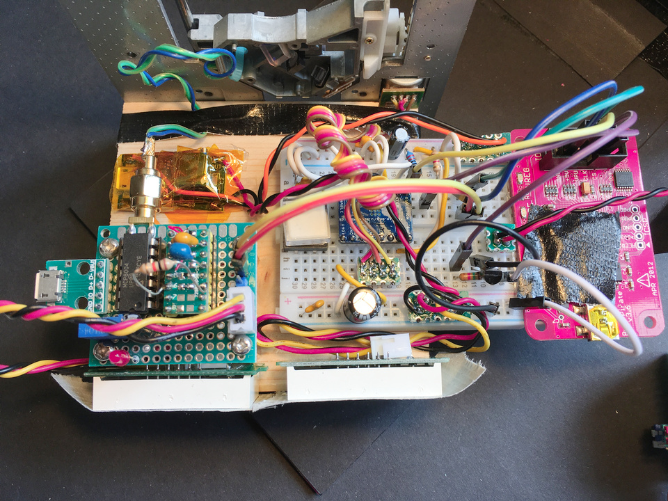 The complete electronics setup. The buspirate on the right interfaces to a computer and controls the
stepper driver and ADC'es the preamp output. The two panel meters show the preamp output and stepper voltage for
setup.
The complete electronics setup. The buspirate on the right interfaces to a computer and controls the
stepper driver and ADC'es the preamp output. The two panel meters show the preamp output and stepper voltage for
setup.
The projection of the spectrum can be adjusted by moving the light source relative to the entry slot and by moving
around the grating DVD.
The capture process
To capture a spectrum, first the light source has to be mounted near the spectrograph's entry slot. The LED tape I
tested I just taped face-down directly into it. Next, the grating DVD has to be adjusted to make sure the spectrum
covers a sensible part of the photodiode's path. Mostly, this boils down to adjusting the photodiode distance and height
to match the vertical extent and wiggling the grating DVD to adjust the projection's horizontal position.
After the optics are set-up, the photodiode preamplifier has to be adjusted. In my experiments, most LED tape at 5GΩ
required a high-ish amplification. The goal in this step is to maximize the peak response of the preamp to be just
shy of its VCC rail to make best use of its dynamic range. To adjust the pre-amp, I took several very coarsely-spaced
measurements to give me an estimate of the peak while I did not yet know its precise location.
Since stray daylight totally swamped out the weak projection of the LED's spectrum I shielded the entire setup with a
small box made of black cardboard and two black t-shirts on top. This shielding proved adequate for all my measurements
but I had to be careful not to accidentially move the DVD that was stuck into the spectrograph with the shielding
t-shirts.
For capturing a single spectrum I wrote a small python script that will automatically move the stepper in adjustable
intervals and take two measurements at each point, one with the LED tape off that can be used for offset calibration and
one with the LED tape on. All measurements are stored in a sqlite database that can then be accesssed from other
scripts.
I built a small script that shows the progress of the current run and an jupyter notebook for data analysis. The jupyter
notebook is capable of live-updating a graph with the in-progress spectrum's data. This was quite useful as a sanity
check for when I made some mistake easy to spot in the resulting data.
After one color channel is captured, the LED tape has to be manually set to the next color and the next measurement can
begin.
 A plot of the raw preamp output voltage versus stepper position. From left to right, the three peaks
are blue, green and red. Step 0 corresponds to the bottommost stepper position and the shortest wavelength.
A plot of the raw preamp output voltage versus stepper position. From left to right, the three peaks
are blue, green and red. Step 0 corresponds to the bottommost stepper position and the shortest wavelength.
Data analysis
Data analysis consists of three major steps: Offset- and stray light removal, wavelength and amplitude calibration and
color space mapping.
Offset removal
The first task is to remove the offset caused by dark current as well as stray light of the LED's bright primary
reflection on the DVD. The LED is very bright and only a small part of its light gets reflected by the grating towards
the photodiode screen. The remaining part of the light is reflected onto the table in front of the DVD spectrograph.
Though I covered all of this with black cardboard, some of that light ultimately gets reflected onto the photodiode.
This causes a large offset, in particular in the blue part of the spectrum since in this part the photodiode is closest
to the spectrograph's opening.
The composite offset can be approximated with a second-order polynomial that is fitted to all the data outside of the
main peak's area. Since at this point the wavelength of each data point is still unknown this is done with a rough first
estimate of the three colors' peaks' locations and widths.
Wavelength- and amplitude calibration
The photodiode's response is strongly wavelength-dependent. In particular in the blue band, the photodiode's sensitivity
gets very poor down to about 20% at the edge to ultraviolet. This effect is strong enough to move the apparent location
of the blue peak towards red.
 A plot of the photodiode's relative sensitivity in the visible spectrum. The sensitivity is
normalized against its peak at 820nm.
A plot of the photodiode's relative sensitivity in the visible spectrum. The sensitivity is
normalized against its peak at 820nm.
The problem is that in order to remove this non-linearity, we would already have to know the wavelength of the measured
light. Since I don't, I settled for a two-step process. First, a coarse wavelength calibration is done relative to the
red peak and the short-wavelength edge of the blue peak. The photodiode measurements are then sensitivity-corrected
using this coarse measurement. Then all three channel peaks are measured in the resulting data and a fine wavelength
estimate is produced by a least-squares fit of a linear function. This fine estimate is then used for a second
sensitivity correction of all original measurements and the scale is changed from stepper motor step count to
wavelength in nanometers.
 A plot of the processed measurements. From left to right, the three peaks are blue, green and red.
Color space mapping
Finally, to achieve the objective of measuring the LED tape's channels' precise color coordinates the measured spetra
have to be matched against the color spaces' color matching functions. The color matching functions describe how
strong the color space's idealized standard observer would react to light at a particular wavelength. Going from a
measured spectrum to color coordinates XYZ works by integrating over the product of the measurement and each color
coordinate's color matching function.
The result are three color coordinates X, Y and Z for each channel R, G and B yielding nine coordinates in total. When
written as a matrix conversion between XYZ color space and LED-RGB color space is as simple as multiplying that matrix
(or its inverse) and a vector from one of the color spaces.
In XYZ space, the set of colors that can be produced with this LED tape is described by the parallelepiped spanned by
the three channel's XYZ vectors. In the following figures, you can see a three-dimensional model of the RGB LED's color
space (colorful) as well as sRGB (white) for comparison plotted within CIE 1931 XYZ. There is no natural map to scale
both so for this illustration the LED color space has been scaled to fit. These figures were made with blender and a few
lines of python. The blender project file including all settings and the python script to generate the color space
models can be found in the project repo.
Illustration of the measured LED color space scaled to fit within XYZ with sRGB (light gray) for
comparison. The thick, white line is the spectral locus.
mkv/h264 download /
webm download
As you can see, the result is pretty disappointing. The LED's color space parallepiped is very narrow, which is because
the blue channel is much brighter than the other two channels. An easy fix for this is to scale-up the RGB space and
drop any values outside XYZ. The scaling factor is a trade-off between color space coverage and brightness. You can
produce the most colors when you clip all channels to brightness of the weakest channel (green in this case), but that
will make the result very dim. Scaling brightness like that stretches the RGB parallelepiped along its major axis. Up to
a point the number of possible colors (the gamut) increases at expense of maximum brightness. When the parallelepiped is
stretched far enought for all three channel vectors to be outside the 1,1,1 XYZ-cube, maximum brightness continues to
decrease but the gamut stays constant. I don't know a simple scientific way to solve this problem, so I just played
around with a couple of factors and settled on 2.5 as a reasonable compromise. Below is an illustration.
Illustration of the measured LED color space at scale factor 2.5 within XYZ with sRGB (light gray)
for comparison. The thick, white line is the spectral locus.
mkv/h264 download /
webm download
Firmware implementation
In the end, the above measurements yield two matrices: One for mapping XYZ to RGB, and one for mapping RGB to XYZ. Of
the several versions of CIE XYZ I chose the CIE 1931 XYZ color space as a basis for the firmware because it is most
popular. Mapping a color coordinate in one color space to the other is as simple as performing nine floating-point
multiplications and six additions. Mapping Lab or Lch to RGB is done by first mapping Lab/Lch to XYZ, then XYZ to RGB.
Lab to XYZ is somewhat complex since it requires a floating-point power for gamma correction, but any self-respecting
libc will have one of those so this is still no problem. Lch also requires floating-point sine and cosine functions, but
these should still be no problem on most hardware.
My implementation of these conversions in the ESP8266 firmware of my Wifi LED driver can be found on Github. You
can view the Jupyter notebook most of the analysis above here.